Data Model
This chapter introduces BanyanDB’s data models and covers the following:
- the high-level data organization
- data model
- data retrieval
You can also find examples of how to interact with BanyanDB using bydbctl, how to create and drop groups, or how to create, read, update and drop streams/measures/traces.
Structure of BanyanDB
The hierarchy that data is organized into streams, measures, traces and properties in groups.
flowchart LR
    G["Group"] --> P["Property (schema-less)"]
    G --> S["Stream"]
    G --> M["Measure"]
    G --> T["Trace"]
    M --> TN["TopNAggregation"]
A group’s catalog fixes which one kind of resource it holds (MEASURE, STREAM, TRACE, or PROPERTY). For how each resource is physically stored on disk, see Storage & File Format.
Groups
Group does not provide a mechanism for isolating groups of resources within a single banyand-server but is the minimal unit to manage physical structures. Each group contains a set of options, like retention policy, shard number, etc. Several shards distribute in a group.
metadata:
  name: others
or
metadata:
  name: sw_metric
catalog: CATALOG_MEASURE
resource_opts:
  shard_num: 2
  segment_interval:
    unit: UNIT_DAY
    num: 1
  ttl:
    unit: UNIT_DAY
    num: 7
The group creates two shards to store data points. Every day, it would create a segment. The available units are HOUR and DAY. The data in this group will keep 7 days.
Every other resource should belong to a group. The catalog indicates which kind of data model the group contains.
Measures
BanyanDB lets you define a measure as follows:
metadata:
  name: service_cpm_minute
  group: sw_metric
tag_families:
  - name: default
    tags:
      - name: id
        type: TAG_TYPE_STRING
      - name: entity_id
        type: TAG_TYPE_STRING
      - name: service_id
        type: TAG_TYPE_STRING
fields:
  - name: total
    field_type: FIELD_TYPE_INT
    encoding_method: ENCODING_METHOD_GORILLA
    compression_method: COMPRESSION_METHOD_ZSTD
  - name: value
    field_type: FIELD_TYPE_INT
    encoding_method: ENCODING_METHOD_GORILLA
    compression_method: COMPRESSION_METHOD_ZSTD
entity:
  tag_names:
    - entity_id
sharding_key:
  tag_names:
    - service_id
index_mode: false
interval: 1m
Measure consists of a sequence of data points. Each data point contains tags and fields.
Tags are key-value pairs. The database engine can index tag values by referring to the index rules and rule bindings, confining the query to filtering data points based on tags bound to an index rule.
Tags are grouped into unique tag_families which are the logical and physical grouping of tags.
Measure supports the following tag types:
- STRING : Text
- INT : 64 bits long integer
- STRING_ARRAY : A group of strings
- INT_ARRAY : A group of integers
- DATA_BINARY : Raw binary
A group of selected tags composite an entity that points out a specific time series the data point belongs to. The database engine has capacities to encode and compress values in the same time series. Users should select appropriate tag combinations to optimize the data size.
To determine the distribution of data across shards, sharding_key can be optionally configured by specifying a set of tags. If sharding_key is not provided, the system will use entity for sharding by default.
Fields are also key-value pairs like tags. But the value of each field is the actual value of a single data point. The database engine would encode and compress the field’s values in the same time series. The query operation is forbidden to filter data points based on a field’s value. You could apply aggregation
functions to them.
Measure supports the following fields types:
- STRING : Text
- INT : 64 bits long integer
- DATA_BINARY : Raw binary
- FLOAT : 64 bits double-precision floating-point number
Measure declares the following encoding/compression options on each field:
- GORILLA (
encoding_method) : a lossless encoding hint for numerical sequences with similar values. - ZSTD (
compression_method) : Zstandard, a real-time compression algorithm with high compression ratios.
How values are actually encoded on disk. These two enums are schema-level hints; the columnar storage engine selects the concrete encoding from the value type and data shape, not from the enum. Numeric (
INT/FLOAT) field columns are delta / delta-of-delta / const encoded with zigzag-varint (floats are first converted to a decimal-int mantissa + exponent); non-numeric columns use dictionary or plain encoding. ZSTD is applied generically by a size threshold (whole index blocks and byte payloads ≥ 128 bytes), not per field. See Storage & File Format for the exact scheme.
Another option named interval indicates the time range between two adjacent data points in a time series and implies that all data points belonging to the same time series are distributed based on a fixed interval. A better practice for naming a measure is to append the interval literal to the tail, for example, service_cpm_minute.
index_mode is a flag to enable the series index as the storage engine. All the tags will be stored in the inverted index and no field is allowed in the measure. This mode is suitable for the non-time series data model but needs TTL to be set. In this mode, the tags defined in the entity is the unique key of the data point. timestamp and version are the common tags in the inverted index.
Same API, two storage engines.
index_modeis the single switch that swaps the entire storage engine behind the sameMeasureschema and the sameWrite/QueryRPCs. Withindex_mode: false, values are stored as columnar parts (the TSDB engine); withindex_mode: true, no columnar part is written at all — the whole data point is stored as a document in the inverted index. The flag is effectively immutable once data exists (flipping it would orphan previously-written data). See Storage & File Format → Measure for the two on-disk layouts.
There is an example of a measure with the index mode enabled:
metadata:
  name: service_traffic
  group: sw_metric
tag_families:
  - name: default
    tags:
      - name: id
        type: TAG_TYPE_STRING
      - name: service_name
        type: TAG_TYPE_STRING
index_mode: true
entity: ["id"]
Measure Registration Operations
TopNAggregation
Find the Top-N entities from a dataset in a time range is a common scenario. We could see the diagrams like “Top 10 throughput endpoints”, and “Most slow 20 endpoints”, etc on SkyWalking’s UI. Exploring and analyzing the top entities can always reveal some high-value information.
BanyanDB introduces the TopNAggregation, aiming to pre-calculate the top/bottom entities during the measure writing phase. In the query phase, BanyanDB can quickly retrieve the top/bottom records. The performance would be much better than top() function which is based on the query phase aggregation procedure.
Caveat:
TopNAggregationis an approximate realization, to use it well you need have a good understanding with the algorithm as well as the data distribution.
---
metadata:
  name: endpoint_cpm_minute_top_bottom
  group: sw_metric
source_measure:
  name: endpoint_cpm_minute
  group: sw_metric
field_name: value
field_value_sort: SORT_UNSPECIFIED
group_by_tag_names:
  - entity_id
counters_number: 1000
lru_size: 10
endpoint_cpm_minute_top_bottom is watching the data ingesting of the source measure endpoint_cpm_minute to generate both top 1000 and bottom 1000 entity cardinalities. If only Top 1000 or Bottom 1000 is needed, the field_value_sort could be DESC or ASC respectively.
- SORT_DESC: Top-N. In a series of
1,2,3...1000. Top10’s result is1000,999...991. - SORT_ASC: Bottom-N. In a series of
1,2,3...1000. Bottom10’s result is1,2...10.
Tags in group_by_tag_names are used as dimensions. These tags can be searched (only equality is supported) in the query phase. Tags do not exist in group_by_tag_names will be dropped in the pre-calculating phase.
counters_number denotes the number of entity cardinality. As the above example shows, calculating the Top 100 among 10 thousands is easier than among 10 millions.
lru_size is a late data optimizing flag. The higher the number, the more late data, but the more memory space is consumed.
TopNAggregation Registration Operations
Streams
Stream shares many details with Measure except for abandoning field. Stream focuses on high throughput data collection, for example, logging. Like Measure, the engine encodes and compresses a stream’s tag columns (delta/dictionary encoding plus zstd for large byte payloads); what Stream lacks is fields (and therefore Measure’s field-level encoding), not encoding altogether. See Storage & File Format → Stream.
Stream Registration Operations
Traces
Trace is a purpose-built data model for distributed tracing data. Unlike Stream, which stores individual elements independently, Trace organizes data around traces — each trace consists of multiple spans that share the same trace ID. The database engine groups spans by trace ID, enabling efficient trace-level queries.
BanyanDB lets you define a trace as follows:
metadata:
  name: sw
  group: sw_trace
tags:
  - name: trace_id
    type: TAG_TYPE_STRING
  - name: state
    type: TAG_TYPE_INT
  - name: service_id
    type: TAG_TYPE_STRING
  - name: service_instance_id
    type: TAG_TYPE_STRING
  - name: endpoint_id
    type: TAG_TYPE_STRING
  - name: duration
    type: TAG_TYPE_INT
  - name: span_id
    type: TAG_TYPE_STRING
  - name: timestamp
    type: TAG_TYPE_TIMESTAMP
trace_id_tag_name: trace_id
span_id_tag_name: span_id
timestamp_tag_name: timestamp
Trace defines a flat list of tags — there are no tag families. Each tag has a name and a type.
Trace supports the following tag types:
- STRING : Text
- INT : 64 bits long integer
- STRING_ARRAY : A group of strings
- INT_ARRAY : A group of integers
- DATA_BINARY : Raw binary
- TIMESTAMP : Timestamp
Three special tag name fields are required:
trace_id_tag_name: Specifies which tag holds the trace ID. The database engine uses this to group spans into traces.span_id_tag_name: Specifies which tag holds the span ID. Each span within a trace has a unique span ID.timestamp_tag_name: Specifies which tag holds the timestamp of the span.
Each data point written to a Trace represents a single span. The database engine automatically groups spans by their trace ID. When querying, the response returns Trace objects, each containing all matching spans that belong to the same trace.
Each span also carries a raw span field (binary), which stores the original span data.
Properties
A Property is a mutable document keyed by group/name/id, stored using a distributed inverted index for efficient tag-based queries. A tag-type contract is registered once via the Property registry, but values are flexible. Unlike Measures, Streams and Traces, a Property is not a time series: it has no timestamp/segment dimension and segment_interval/ttl do not apply; updates overwrite by ModRevision (last-writer-wins) and deletes are soft (tombstoned, reclaimed lazily at merge). See Storage & File Format → Property.
We should create a group before creating a property.
Creating group.
metadata:
  name: sw
catalog: CATALOG_PROPERTY
resource_opts:
  shard_num: 2
Creating property.
metadata:
  container:
    group: sw
    name: temp_data
  id: General-Service
tags:
  - key: name
    value:
      str:
        value: "hello"
  - key: state
    value:
      str:
        value: "succeed"
Property supports a three-level hierarchy, group/name/id, that is more flexible than schemaful data models.
Data Models
Data models in BanyanDB derive from some classic data models.
TimeSeries Model
A time series is a series of data points indexed in time order. Most commonly, a time series is a sequence taken at successive equally spaced points in time. Thus it is a sequence of discrete-time data.
You can store time series data points through Stream, Measure or Trace. Examples of Stream are logs and events. Trace is designed for distributed tracing data. Measure could ingest metrics, profiles, etc.
Key-Value Model
The key-value data model is a subset of the Property data model. Every property has a key <group>/<name>/<id> that identifies a property within a collection. This key acts as the primary key to retrieve the data. You can set it when creating a key. It cannot be changed later because the attribute is immutable.
There are several Key-Value pairs in a property, named Tags. You could add, update and drop them based on the tag’s key.
Data Retrieval
Queries and Writes are used to filter schemaful data models, Stream, Measure, Trace or TopNAggregation based on certain criteria, as well as to compute or store new data.
MeasureServiceprovidesWrite,QueryandTopNStreamServiceprovidesWrite,QueryTraceServiceprovidesWrite,Query
Query Projection Flexibility
As of 0.10.0, tags used in query criteria (the WHERE clause) no longer need to be included in the projection (the SELECT clause). Previously, any tag referenced in a filter condition had to also appear in the result projection. This restriction has been removed, allowing more flexible queries.
For example, the following query filters on service_id but only projects duration:
SELECT duration
FROM MEASURE service_latency IN production
TIME > '-30m'
WHERE service_id = 'frontend';
This applies to queries across Stream, Measure, and Trace data models.
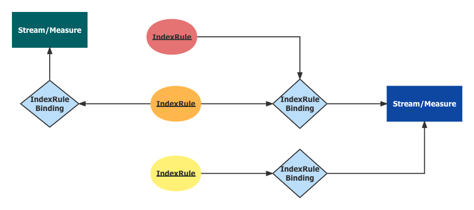
IndexRule & IndexRuleBinding
An IndexRule indicates which tags are indexed. An IndexRuleBinding binds an index rule to the target resources or the subject. There might be several rule bindings to a single resource, but their effective time range could NOT overlap.
metadata:
  name: trace_id
  group: sw_stream
tags:
  - trace_id
type: TYPE_INVERTED
IndexRule supports several kinds of index structures. The INVERTED index is suitable for measure tag indexing due to better query performance. The SKIPPING index is optimized for the majority of stream tags, which prioritizes efficient space utilization. The TREE index is designed for trace, which stores data with user-controlled int64 ordering keys (e.g., duration, timestamp) in a tree index, enabling efficient sorted result retrieval on numeric tags.
metadata:
  name: stream_binding
  group: sw_stream
rules:
  - trace_id
  - duration
  - endpoint_id
  - status_code
  - http.method
  - db.instance
  - db.type
  - mq.broker
  - mq.queue
  - mq.topic
  - extended_tags
subject:
  catalog: CATALOG_STREAM
  name: sw
begin_at: "2021-04-15T01:30:15.01Z"
expire_at: "2121-04-15T01:30:15.01Z"
IndexRuleBinding binds IndexRules to a subject, Stream, Measure or Trace. The time range between begin_at and expire_at is the effective time.
IndexRule Registration Operations
IndexRuleBinding Registration Operations
Index Granularity
In BanyanDB, Stream, Measure and Trace have different levels of index granularity.
For Measure, the indexed target is a data point with specific tag values. The query processor uses the tag values defined in the entity field of the Measure to compose a series ID, which is used to find the several series that match the query criteria. The entity field is a set of tags that defines the unique identity of a time series, and it restricts the tags that can be used as indexed target.
Each series contains a sequence of data points that share the same tag values. Once the query processor has identified the relevant series, it scans the data points between the desired time range in those series to find the data that matches the query criteria.
For example, suppose we have a Measure with the following entity field: {service, operation, instance}. If we get a data point with the following tag values: service=shopping, operation=search, and instance=prod-1, then the query processor would use those tag values to construct a series ID that uniquely identifies the series containing that data point. The query processor would then scan the relevant data points in that series to find the data that matches the query criteria.
The side effect of the measure index is that each indexed value has to represent a unique seriesID. This is because the series ID is constructed by concatenating the indexed tag values in the entity field. If two series have the same entity field, they would have the same series ID and would be indistinguishable from one another. This means that if you want to index a tag that is not part of the entity field, you would need to ensure that it is unique across all series. One way to do this would be to include the tag in the entity field, but this may not always be feasible or desirable depending on your use case.
For Stream, the indexed target is an element that is a combination of the series ID and timestamp. The Stream query processor uses the time range to find target files. The indexed result points to the target element. The processor doesn’t have to scan a series of elements in this time range, which reduces the query time.
For example, suppose we have a Stream with the following tags: service, operation, instance, and status_code. If we get a data point with the following tag values: service=shopping, operation=search, instance=prod-1, and status_code=200, and the data point’s time is 1:00pm on January 1st, 2022, then the series ID for this data point would be shopping_search_prod-1_200_1641052800, where 1641052800 is the Unix timestamp representing 1:00pm on January 1st, 2022.
The indexed target would be the combination of the series ID and timestamp, which in this case would be shopping_search_prod-1_200_1641052800. The Stream query processor would use the time range specified in the query to find target files and then search within those files for the indexed target.
For Trace, the indexed target is a numeric tag value stored in a tree index via TREE type index rules. The tree index maintains data ordered by user-controlled int64 keys, enabling efficient sorted queries on numeric tags such as duration. When a TREE index rule is bound to a trace, the database engine extracts the int64 value from the indexed tag and uses it as the ordering key. This allows queries to efficiently retrieve and sort traces by numeric dimensions without scanning all data.
For example, suppose we have a Trace with a TREE index rule bound to the duration tag. If a span has duration=350, the tree index stores this value as the ordering key pointing to that span. When querying for traces with duration > 200, the tree index directly locates the matching entries by performing an ordered range scan, avoiding full data scans.
The following is a comparison of the indexing granularity, performance, and flexibility of Measure, Stream and Trace indices:
| Type | Indexing Granularity | Performance | Flexibility |
|---|---|---|---|
| Measure | Indices are constructed for each series and are based on the entity field of the Measure. Each indexed value has to represent a unique seriesID. | Fast for lookups due to series-level indexing. | Less flexible; requires care when indexing tags that are not part of the entity field. |
| Stream | Indices are constructed for each element and are based on the series ID and timestamp. | Slower than Measure due to element-level indexing. | More flexible than Measure; can index any tag value. |
| Trace | Indices are constructed per element using a tree index, ordered by int64 tag values. | Efficient for sorted retrieval on numeric tags. | Limited to int64/timestamp tags with TREE type index rules; does not support inverted or skipping indices. |
In general, Measure indices are fast and efficient, but they require more care when indexing tags that are not part of the entity field. Stream indices are slower and take up more space, but they can index any tag value and do not have the same side effects as Measure indices. Trace indices excel at sorted queries on numeric dimensions, but are limited to TREE type index rules with int64 or timestamp tag values.