Diagnose Service Mesh Network Performance with eBPF
Background
This article will show how to use Apache SkyWalking with eBPF to make network troubleshooting easier in a service mesh environment.
Apache SkyWalking is an application performance monitor tool for distributed systems. It observes metrics, logs, traces, and events in the service mesh environment and uses that data to generate a dependency graph of your pods and services. This dependency graph can provide quick insights into your system, especially when there’s an issue.
However, when troubleshooting network issues in SkyWalking’s service topology, it is not always easy to pinpoint where the error actually is. There are two reasons for the difficulty:
- Traffic through the Envoy sidecar is not easy to observe. Data from Envoy’s Access Log Service (ALS) shows traffic between services (sidecar-to-sidecar), but not metrics on communication between the Envoy sidecar and the service it proxies. Without that information, it is more difficult to understand the impact of the sidecar.
- There is a lack of data from transport layer (OSI Layer 4) communication. Since services generally use application layer (OSI Layer 7) protocols such as HTTP, observability data is generally restricted to application layer communication. However, the root cause may actually be in the transport layer, which is typically opaque to observability tools.
Access to metrics from Envoy-to-service and transport layer communication can make it easier to diagnose service issues. To this end, SkyWalking needs to collect and analyze transport layer metrics between processes inside Kubernetes pods - a task well suited to eBPF. We investigated using eBPF for this purpose and present our results and a demo below.
Monitoring Kubernetes Networks with eBPF
With its origins as the Extended Berkeley Packet Filter, eBPF is a general purpose mechanism for injecting and running your own code into the Linux kernel and is an excellent tool for monitoring network traffic in Kubernetes Pods. In the next few sections, we'll provide an overview of how to use eBPF for network monitoring as background for introducing Skywalking Rover, a metrics collector and profiler powered by eBPF to diagnose CPU and network performance.
How Applications and the Network Interact
Interactions between the application and the network can generally be divided into the following steps from higher to lower levels of abstraction:

- User Code: Application code uses high-level network libraries in the application stack to exchange data across the network, like sending and receiving HTTP requests.
- Network Library: When the network library receives a network request, it interacts with the language API to send the network data.
- Language API: Each language provides an API for operating the network, system, etc. When a request is received, it interacts with the system API. In Linux, this API is called syscalls.
- Linux API: When the Linux kernel receives the request through the API, it communicates with the socket to send the data, which is usually closer to an OSI Layer 4 protocol, such as TCP, UDP, etc.
- Socket Ops: Sending or receiving the data to/from the NIC.
Our hypothesis is that eBPF can monitor the network. There are two ways to implement the interception: User space (uprobe) or Kernel space (kprobe). The table below summarizes the differences.
| Pros | Cons | |
|---|---|---|
| uprobe | • Get more application-related contexts, such as whether the current request is HTTP or HTTPS.• Requests and responses can be intercepted by a single method | • Data structures can be unstable, so it is more difficult to get the desired data. • Implementation may differ between language/library versions. • Does not work in applications without symbol tables. |
| kprobe | • Available for all languages. • The data structure and methods are stable and do not require much adaptation. • Easier correlation with underlying data, such as getting the destination address of TCP, OSI Layer 4 protocol metrics, etc. | • A single request and response may be split into multiple probes. • Contextual information is not easy to get for stateful requests. For example header compression in HTTP/2. |
For the general network performance monitor, we chose to use the kprobe (intercept the syscalls) for the following reasons:
- It’s available for applications written in any programming language, and it’s stable, so it saves a lot of development/adaptation costs.
- It can be correlated with metrics from the system level, which makes it easier to troubleshoot.
- As a single request and response are split into multiple probes, we can use technology to correlate them.
- For contextual information, It’s usually used in OSI Layer 7 protocol network analysis. So, if we just monitor the network performance, then they can be ignored.
Kprobes and network monitoring
Following the network syscalls of Linux documentation, we can implement network monitoring by intercepting two types of methods: socket operations and send/receive methods.
Socket Operations
When accepting or connecting with another socket, we can get the following information:
- Connection information: Includes the remote address from the connection which helps us to understand which pod is connected.
- Connection statics: Includes basic metrics from sockets, such as round-trip time (RTT), lost packet count in TCP, etc.
- Socket and file descriptor (FD) mapping: Includes the relationship between the Linux file descriptor and socket object. It is useful when sending and receiving data through a Linux file descriptor.
Send/Receive
The interface related to sending or receiving data is the focus of performance analysis. It mainly contains the following parameters:
- Socket file descriptor: The file descriptor of the current operation corresponding to the socket.
- Buffer: The data sent or received, passed as a byte array.
Based on the above parameters, we can analyze the following data:
- Bytes: The size of the packet in bytes.
- Protocol: The protocol analysis according to the buffer data, such as HTTP, MySQL, etc.
- Execution Time: The time it takes to send/receive the data.
At this point (Figure 1) we can analyze the following steps for the whole lifecycle of the connection:
- Connect/Accept: When the connection is created.
- Transform: Sending and receiving data on the connection.
- Close: When the connection is closed.

Figure 1
Protocol and TLS
The previous section described how to analyze connections using send or receive buffer data. For example, following the HTTP/1.1 message specification to analyze the connection. However, this does not work for TLS requests/responses.

Figure 2
When TLS is in use, the Linux Kernel transmits data encrypted in user space. In the figure above, The application usually transmits SSL data through a third-party library (such as OpenSSL). For this case, the Linux API can only get the encrypted data, so it cannot recognize any higher layer protocol. To decrypt inside eBPF, we need to follow these steps:
- Read unencrypted data through uprobe: Compatible multiple languages, using uprobe to capture the data that is not encrypted before sending or after receiving. In this way, we can get the original data and associate it with the socket.
- Associate with socket: We can associate unencrypted data with the socket.
OpenSSL Use case
For example, the most common way to send/receive SSL data is to use OpenSSL as a shared library, specifically the SSL_read and SSL_write methods to submit the buffer data with the socket.
Following the documentation, we can intercept these two methods, which are almost identical to the API in Linux. The source code of the SSL structure in OpenSSL shows that the Socket FD exists in the BIO object of the SSL structure, and we can get it by the offset.
In summary, with knowledge of how OpenSSL works, we can read unencrypted data in an eBPF function.
Introducing SkyWalking Rover, an eBPF-based Metrics Collector and Profiler
SkyWalking Rover introduces the eBPF network profiling feature into the SkyWalking ecosystem. It’s currently supported in a Kubernetes environment, so must be deployed inside a Kubernetes cluster. Once the deployment is complete, SkyWalking Rover can monitor the network for all processes inside a given Pod. Based on the monitoring data, SkyWalking can generate the topology relationship diagram and metrics between processes.
Topology Diagram
The topology diagram can help us understand the network access between processes inside the same Pod, and between the process and external environment (other Pod or service). Additionally, it can identify the data direction of traffic based on the line flow direction.
In Figure 3 below, all nodes within the hexagon are the internal process of a Pod, and nodes outside the hexagon are externally associated services or Pods. Nodes are connected by lines, which indicate the direction of requests or responses between nodes (client or server). The protocol is indicated on the line, and it’s either HTTP(S), TCP, or TCP(TLS). Also, we can see in this figure that the line between Envoy and Python applications is bidirectional because Envoy intercepts all application traffic.
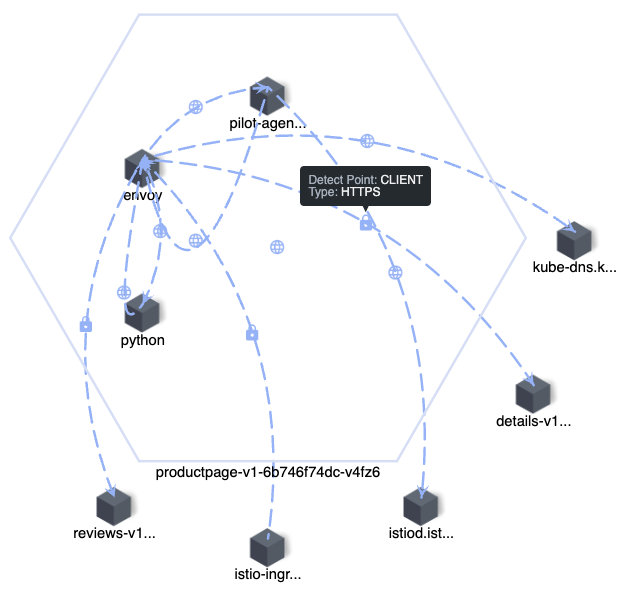
Figure 3
Metrics
Once we recognize the network call relationship between processes through the topology, we can select a specific line and view the TCP metrics between the two processes.
The diagram below (Figure 4) shows the metrics of network monitoring between two processes. There are four metrics in each line. Two on the left side are on the client side, and two on the right side are on the server side. If the remote process is not in the same Pod, only one side of the metrics is displayed.
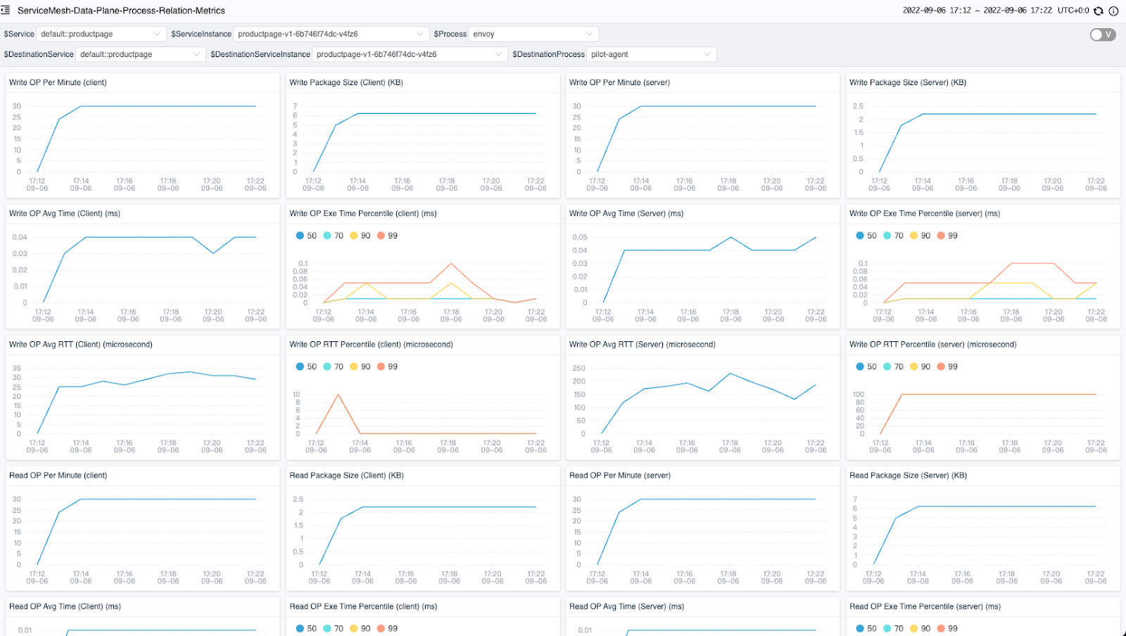
Figure 4
The following two metric types are available:
- Counter: Records the total number of data in a certain period. Each counter contains the following data: a. Count: Execution count. b. Bytes: Packet size in bytes. c. Execution time: Execution duration.
- Histogram: Records the distribution of data in the buckets.
Based on the above data types, the following metrics are exposed:
| Name | Type | Unit | Description |
|---|---|---|---|
| Write | Counter and histogram | Millisecond | The socket write counter. |
| Read | Counter and histogram | Millisecond | The socket read counter. |
| Write RTT | Counter and histogram | Microsecond | The socket write round trip time (RTT) counter. |
| Connect | Counter and histogram | Millisecond | The socket connect/accept with another server/client counter. |
| Close | Counter and histogram | Millisecond | The socket with other socket counter. |
| Retransmit | Counter | Millisecond | The socket retransmit package counter. |
| Drop | Counter | Millisecond | The socket drop package counter. |
Demo
In this section, we demonstrate how to perform network profiling in the service mesh. To follow along, you will need a running Kubernetes environment.
NOTE: All commands and scripts are available in this GitHub repository.
Install Istio
Istio is the most widely deployed service mesh, and comes with a complete demo application that we can use for testing. To install Istio and the demo application, follow these steps:
- Install Istio using the demo configuration profile.
- Label the default namespace, so Istio automatically injects Envoy sidecar proxies when we’ll deploy the application.
- Deploy the bookinfo application to the cluster.
- Deploy the traffic generator to generate some traffic to the application.
export ISTIO_VERSION=1.13.1

# install istio
istioctl install -y --set profile=demo
kubectl label namespace default istio-injection=enabled

# deploy the bookinfo applications
kubectl apply -f https://raw.githubusercontent.com/istio/istio/$ISTIO_VERSION/samples/bookinfo/platform/kube/bookinfo.yaml
kubectl apply -f https://raw.githubusercontent.com/istio/istio/$ISTIO_VERSION/samples/bookinfo/networking/bookinfo-gateway.yaml
kubectl apply -f https://raw.githubusercontent.com/istio/istio/$ISTIO_VERSION/samples/bookinfo/networking/destination-rule-all.yaml
kubectl apply -f https://raw.githubusercontent.com/istio/istio/$ISTIO_VERSION/samples/bookinfo/networking/virtual-service-all-v1.yaml

# generate traffic
kubectl apply -f https://raw.githubusercontent.com/mrproliu/skywalking-network-profiling-demo/main/resources/traffic-generator.yaml
Install SkyWalking
The following will install the storage, backend, and UI needed for SkyWalking:
git clone https://github.com/apache/skywalking-helm.git
cd skywalking-helm
cd chart
helm dep up skywalking
helm -n istio-system install skywalking skywalking \
 --set fullnameOverride=skywalking \
 --set elasticsearch.minimumMasterNodes=1 \
 --set elasticsearch.imageTag=7.5.1 \
 --set oap.replicas=1 \
 --set ui.image.repository=apache/skywalking-ui \
 --set ui.image.tag=latest \
 --set oap.image.tag=9.2.0 \
 --set oap.envoy.als.enabled=true \
 --set oap.image.repository=apache/skywalking-oap-server \
 --set oap.storageType=elasticsearch \
 --set oap.env.SW_METER_ANALYZER_ACTIVE_FILES='network-profiling'
Install SkyWalking Rover
SkyWalking Rover is deployed on every node in Kubernetes, and it automatically detects the services in the Kubernetes cluster. The network profiling feature has been released in the version 0.3.0 of SkyWalking Rover. When a network monitoring task is created, the SkyWalking rover sends the data to the SkyWalking backend.
kubectl apply -f https://raw.githubusercontent.com/mrproliu/skywalking-network-profiling-demo/main/resources/skywalking-rover.yaml
Start the Network Profiling Task
Once all deployments are completed, we must create a network profiling task for a specific instance of the service in the SkyWalking UI.
To open SkyWalking UI, run:
kubectl port-forward svc/skywalking-ui 8080:80 --namespace
istio-system
Currently, we can select the specific instances that we wish to monitor by clicking the Data Plane item in the Service Mesh panel and the Service item in the Kubernetes panel.
In the figure below, we have selected an instance with a list of tasks in the network profiling tab. When we click the start button, the SkyWalking Rover starts monitoring this instance’s network.
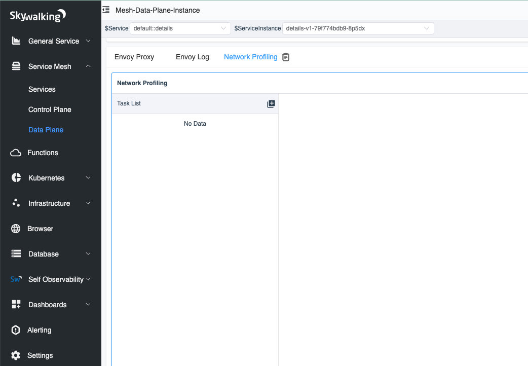
Figure 5
Done!
After a few seconds, you will see the process topology appear on the right side of the page.
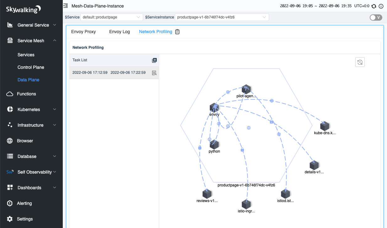
Figure 6
When you click on the line between processes, you can see the TCP metrics between the two processes.
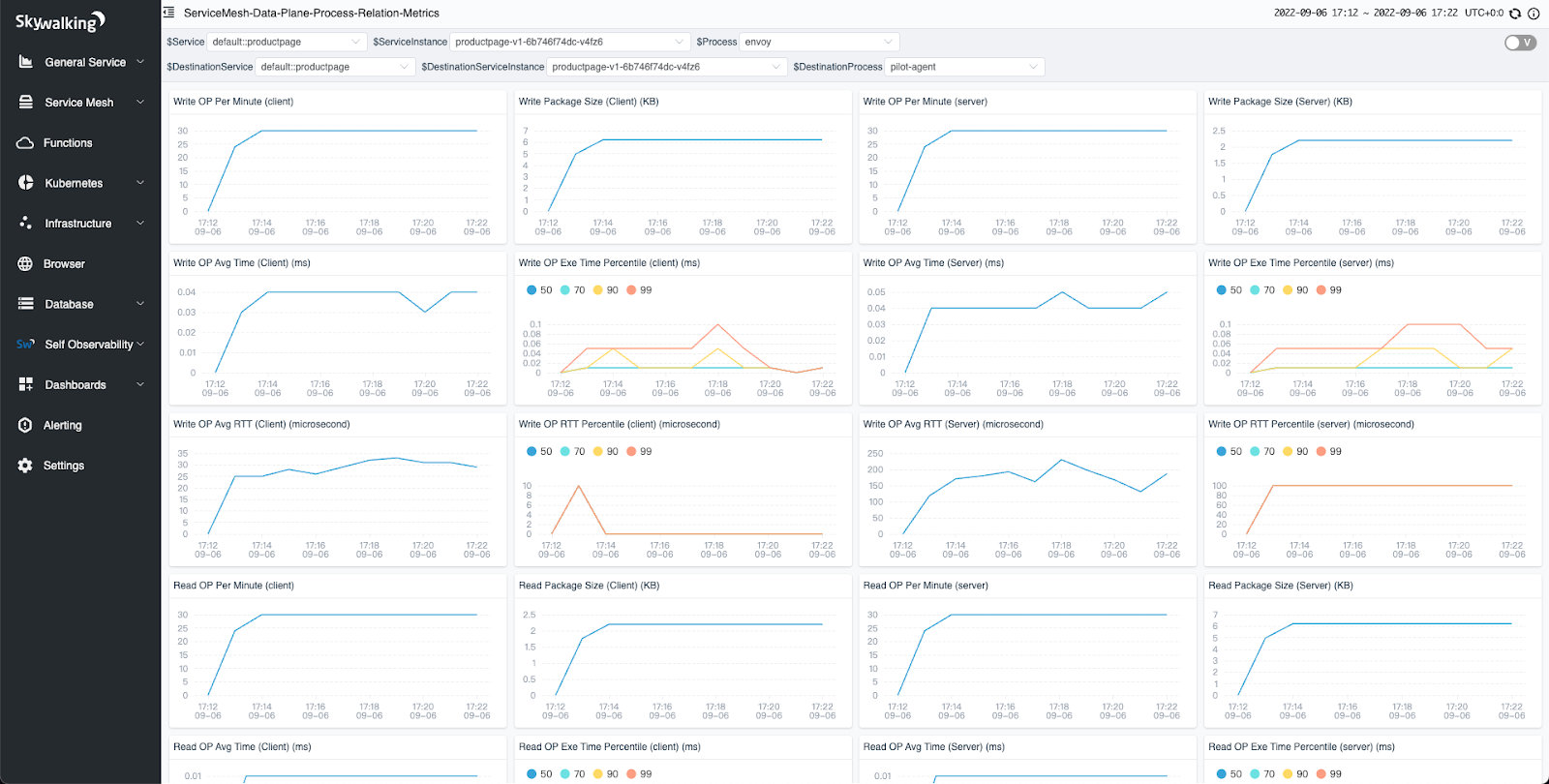
Figure 7
Conclusion
In this article, we detailed a problem that makes troubleshooting service mesh architectures difficult: lack of context between layers in the network stack. These are the cases when eBPF begins to really help with debugging/productivity when existing service mesh/envoy cannot. Then, we researched how eBPF could be applied to common communication, such as TLS. Finally, we demo the implementation of this process with SkyWalking Rover.
For now, we have completed the performance analysis for OSI layer 4 (mostly TCP). In the future, we will also introduce the analysis for OSI layer 7 protocols like HTTP.