Meet Horizon UI · 11/17: Runtime Rules & Live Debugging
This is the eleventh post in the Meet Horizon UI series, and it stays in Act 3 — operate it. The previous post was about reading what the backend already decided; this one is about changing how it decides — and then proving the change does what you meant.
Almost everything OAP computes runs through a small family of DSLs: OAL turns traces into service and endpoint metrics, MAL turns meters (OpenTelemetry, Telegraf) into metrics, LAL turns logs into tags and metrics. Traditionally you edit those as YAML on the server and restart. Horizon brings both halves into the console — edit and hot-apply the rules, and debug them against live data — two capabilities new to the SkyWalking UI that ride OAP’s admin host.
Your rules, live in the console
Operate → DSL management lists every analysis rule the cluster is running, grouped by source. Four catalogs are editable — MAL · OTel, MAL · Telegraf, LAL, and LAL → MAL (log-to-metric) — plus a read-only OAL browser. Rules group by prefix (ActiveMQ, BanyanDB, Elasticsearch, Flink…), each tagged by status, and you can filter by active / inactive / bundled / modified to see at a glance what an operator has changed versus what shipped.
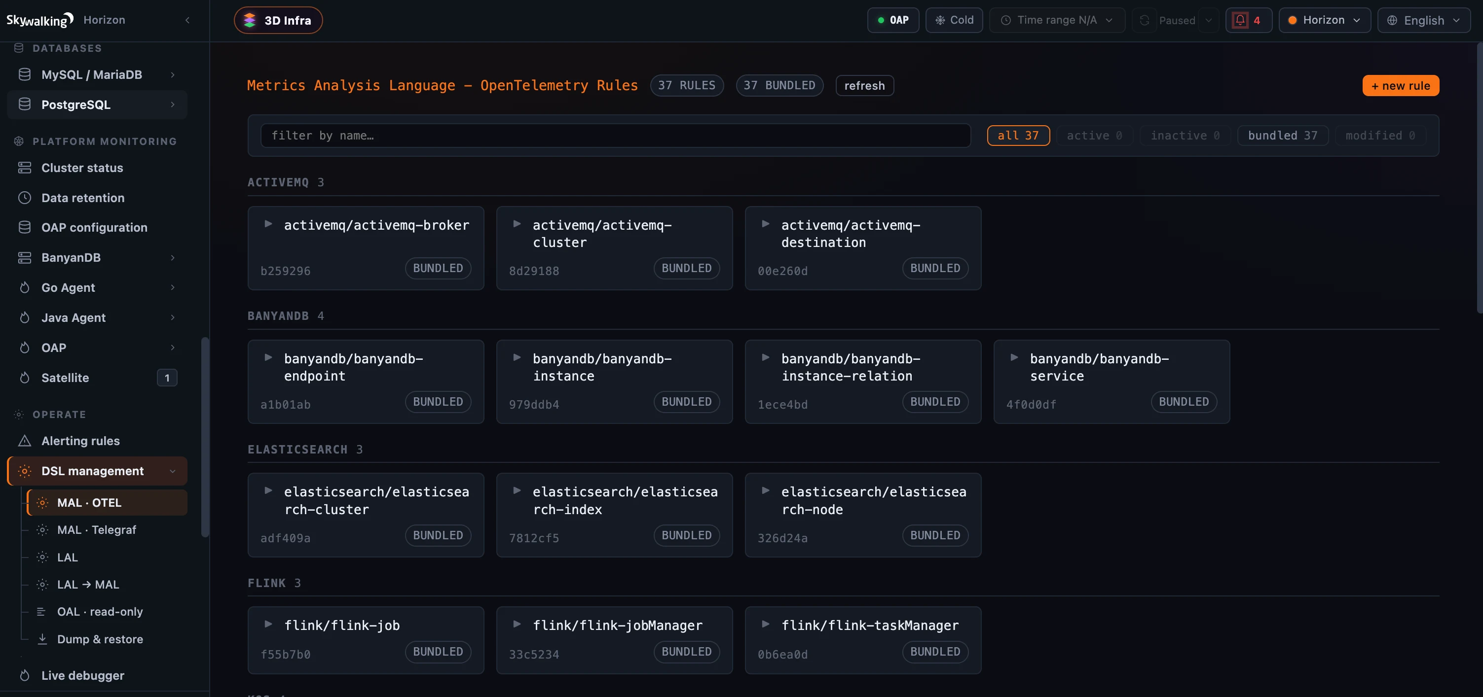 Figure 1: DSL management — every OAL/MAL/LAL rule the cluster runs, grouped by source and filterable by status (active / inactive / bundled / modified). Here, the OpenTelemetry MAL catalog: 37 bundled rules.
Edit, and hot-apply safely
Open a rule and it’s a Monaco YAML editor with syntax highlighting and two diff modes — vs. server (what’s live) and vs. bundled (what shipped) — so you always see what you’re about to change. The green ▶ in the gutter beside each - name: jumps that rule straight into the Live Debugger.
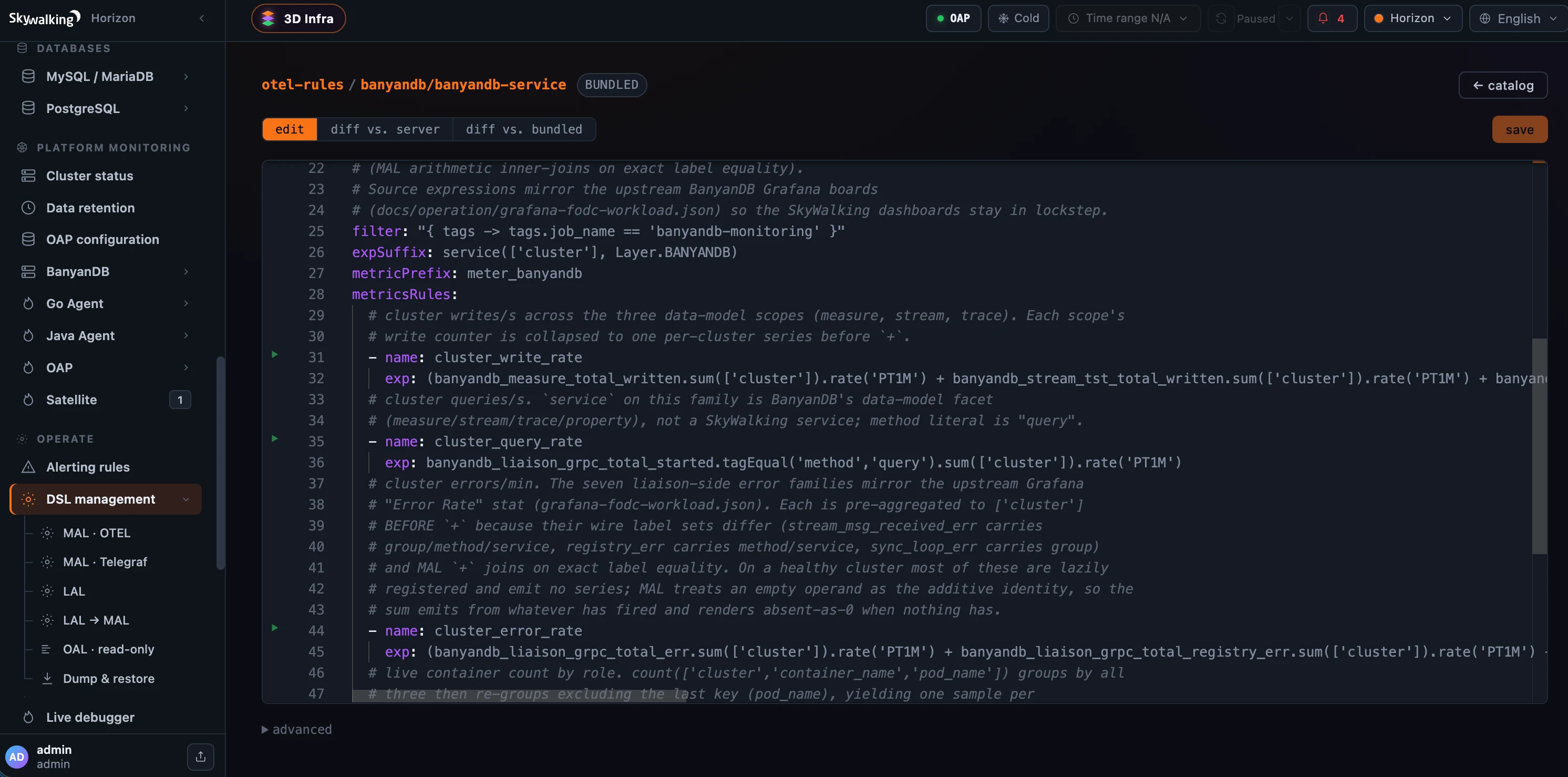 Figure 2: Edit a rule as Monaco YAML — syntax-highlighted, with diffs against the live (server) and bundled versions, and a green ▶ in the gutter that jumps the rule into the Live Debugger.
Saving is where the care shows. A body- or filter-only edit applies instantly. But a structural change — one that moves a metric’s scope, downsampling, or storage shape — reshapes the cluster’s storage, so Horizon runs it as a fenced rollout and tracks it on screen: Compiled → Confirming across the cluster → Committing → Done, reporting success only once the change is durable. If a node lags the fence, the apply ends DEGRADED — it names the laggard nodes (they self-converge on their next scan) rather than failing; a pre-commit error is rolled back with the reason inline and your edit kept in the buffer; a compile error surfaces as an inline diagnostic. A one-click Force re-apply re-runs a stuck rollout on byte-identical content to un-stick a node (it briefly pauses that one rule’s collection). Reverting a rule to its bundled default goes through the same fenced path; you can also inactivate it, delete it, or dump the whole catalog to a tarball.
The Live Debugger: see what a rule actually does
Editing a rule is the easy part. The hard part — the part that used to mean reading code and squinting at output — is knowing what a rule computes against your real data. Operate → Live debugger answers that directly: pick a rule, click start sampling, and Horizon installs a bounded capture on every reachable OAP node, grabs a handful of real records, and shows each one stepped through the rule.
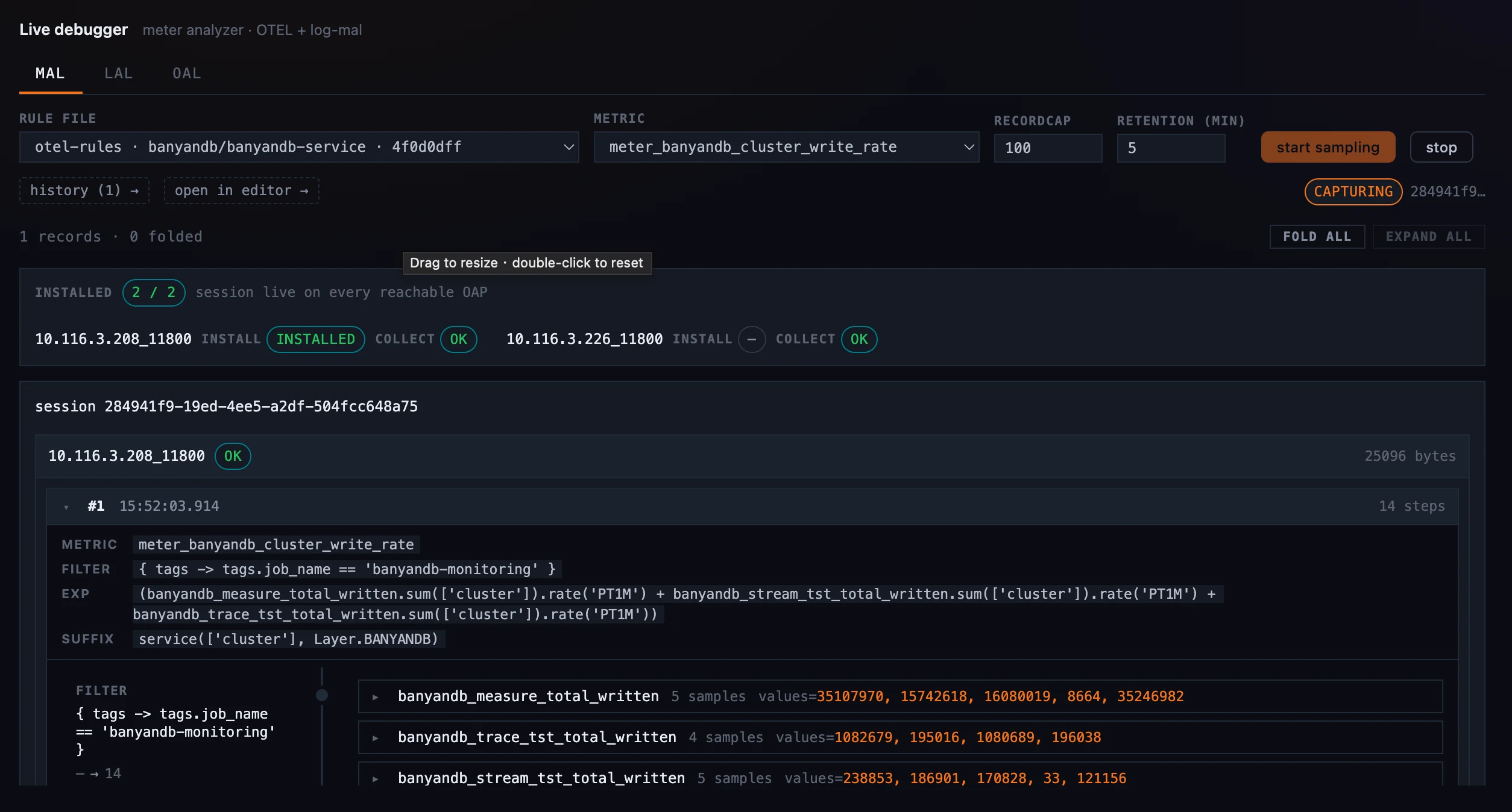 Figure 3: Start a capture and it installs on every reachable OAP node (here 2/2), grabs real records, and bounds itself with a record cap and a retention window — the same shell serves all three analysis languages.
It has one tab per analysis language, because each works on a different kind of data.
OAL → traces. A captured source row — a real trace segment — flows clause by clause: from(Service.*) reads the segment (you see its latency, status, endpoint), build_metrics shapes it, cpm() aggregates it. You watch a trace become a metric.
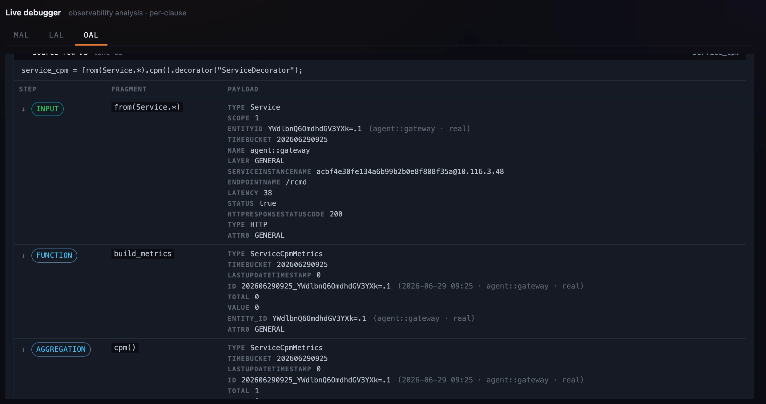 Figure 4: OAL → traces — a real segment from
 agent::gateway (latency 38, status 200, /rcmd) stepped clause by clause, from(Service.*) → build_metrics → cpm(), into the service-CPM metric it feeds.
MAL → metrics. A meter sample flows input → filter → function → output. Because one metric fans out into many label-sets, the samples are grouped by metric, and a diff dims the labels every sample shares and highlights only the ones that differ.
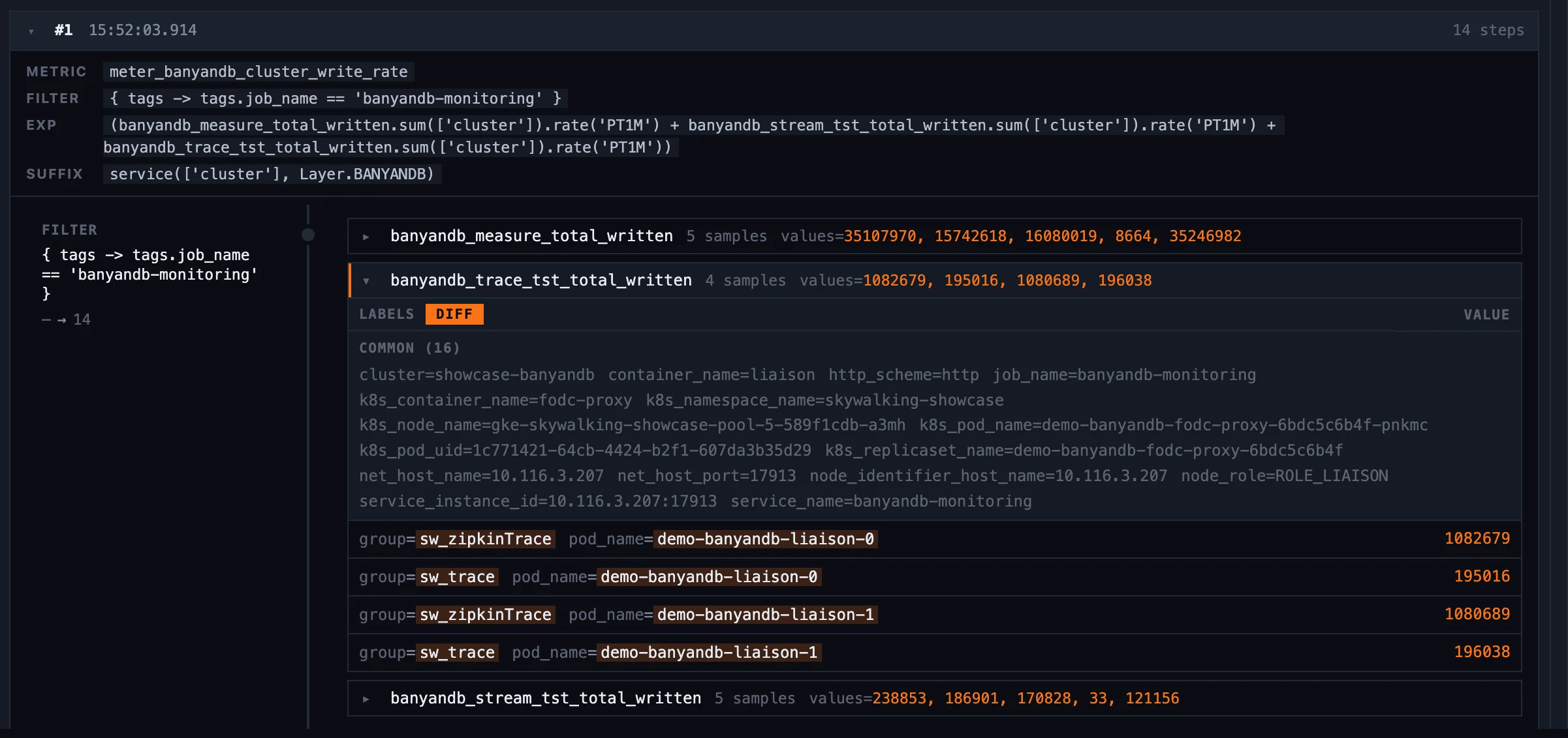 Figure 5: MAL → metrics — samples grouped by metric, with a diff that dims the 16 labels every sample shares and lights only the two that differ (
group, pod_name), so four near-identical series read apart at a glance.
LAL → logs. Each captured log record becomes a column and each DSL block (or statement) a row, so the whole capture reads as a matrix: you can see which records the filter aborted and what the extractor pulled out of the ones that passed — and click any cell to open the record in full and compare it against another.
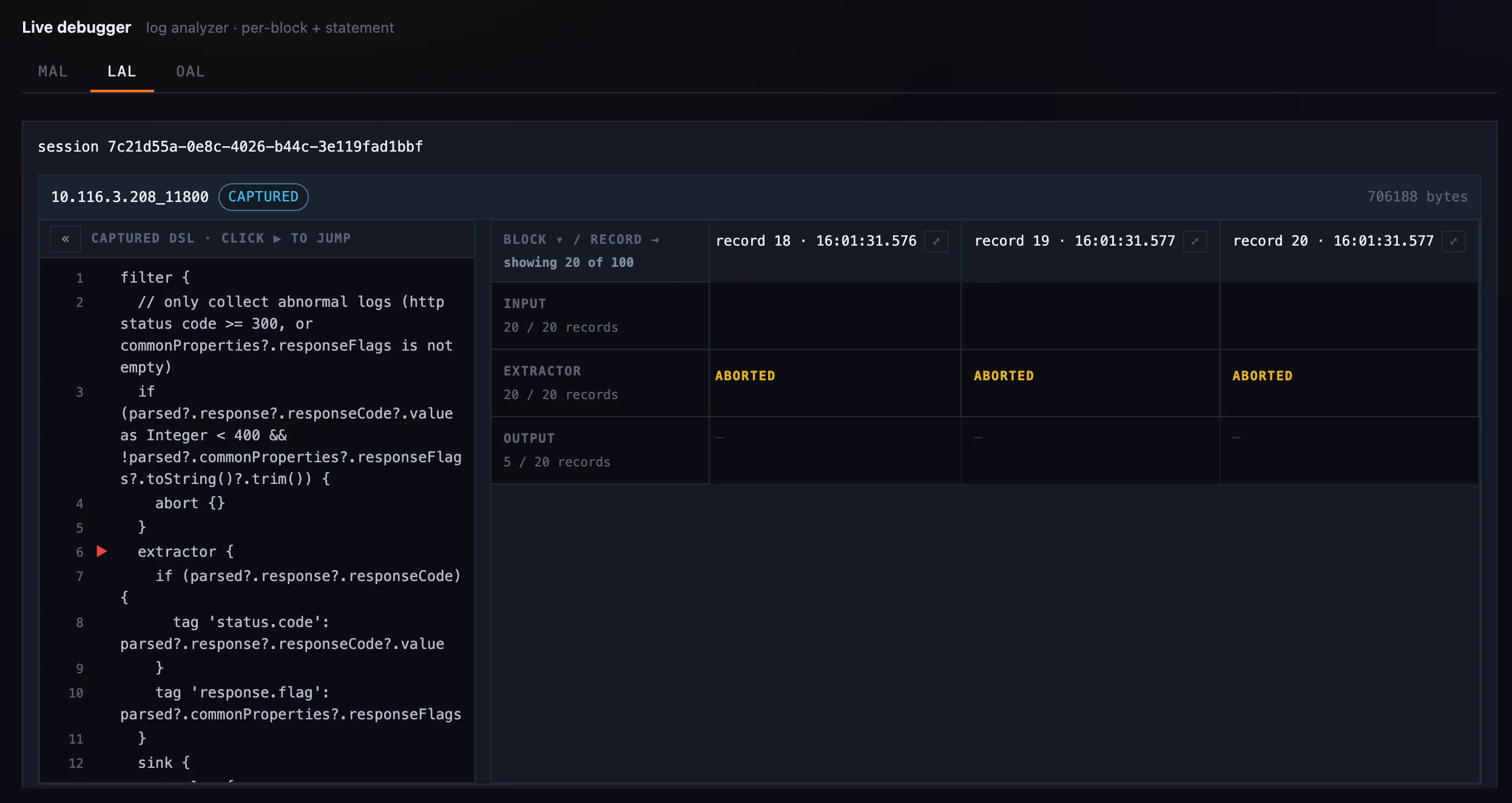 Figure 6: LAL → logs — every captured record is a column, every DSL block a row. The
 filter aborts the normal logs; for each abnormal one that passes, the extractor row shows the tag it added (status.code=404) as a diff over the raw record.
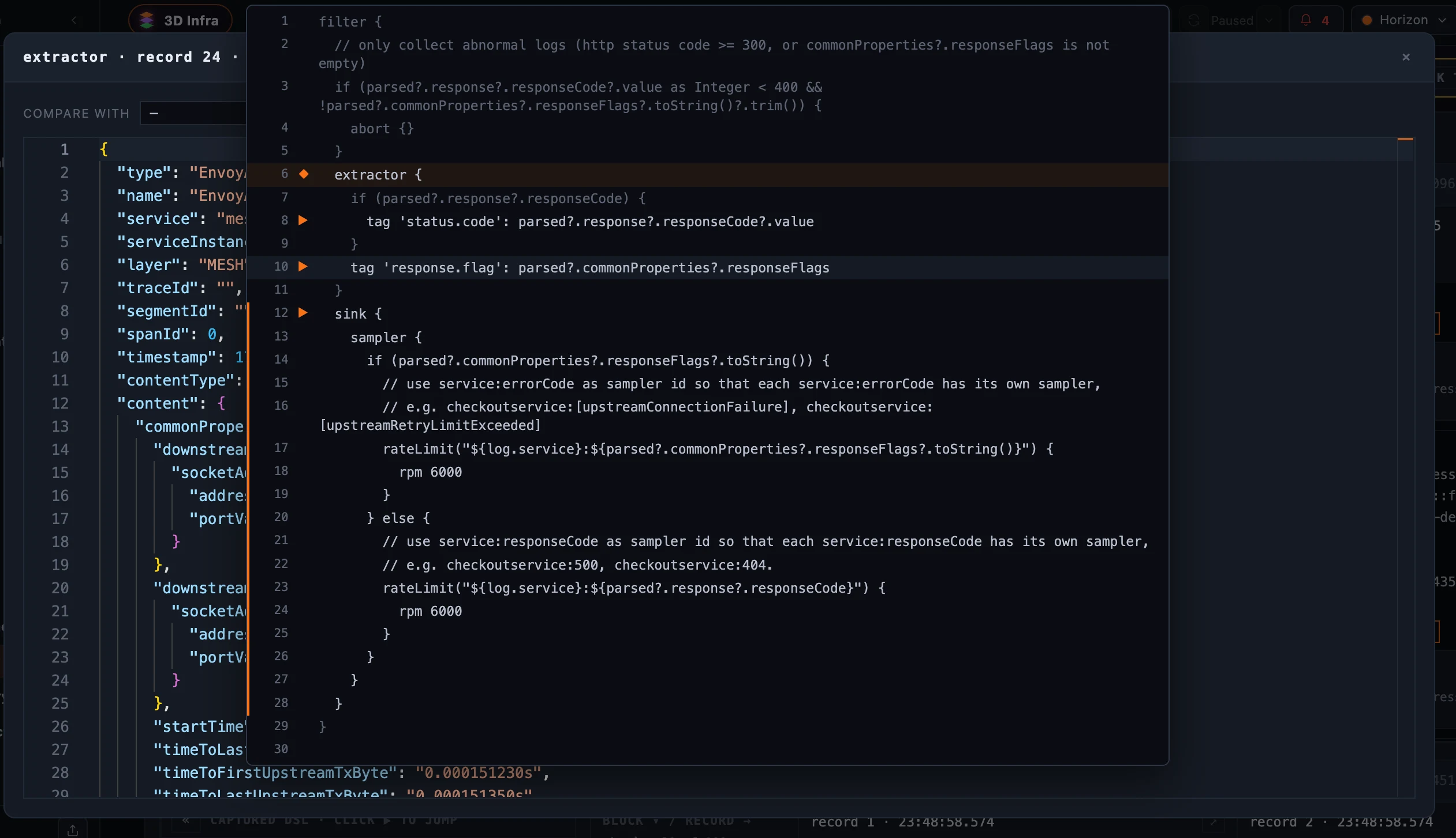 Figure 7: “Show complete data” opens a record in full — the entire raw log payload (here an Envoy access log) — with a Compare with selector to diff it field-by-field against any other captured record.
Where it runs
Both surfaces are operate features: they talk to OAP’s admin host, not the query port — DSL management through the receiver-runtime-rule module, the Live Debugger through dsl-debugging. That admin host ships with OAP 11, so on today’s backend these two pages surface a clear “needs the admin host / module” banner and stay read-only, while every observe surface — dashboards, traces, logs, alarms, profiling — keeps working untouched. Access is role-gated: browsing rules and viewing captures are read permissions, while editing, structural apply, and running a capture each need their own write or execute verb — so a read-only operator can study captured samples all day without ever being able to change a rule or start a session. This is the slice of “operate” the open-source backend only just made possible.
Where to go next
For the field reference — every apply state, the dump format, the per-tab capture controls — see the Runtime Rules and Live Debugger docs.
Next up: Inspect — Cross-Layer Query Power-Tools — the Operate-side surfaces for running metric, trace, and log queries straight across every layer.