Meet Horizon UI · 9/17: Five Profilers, One Flame Graph
This is the ninth post in the Meet Horizon UI series. Metrics tell you what slowed down; traces tell you which hop. Profiling goes one level deeper — into the call stacks, kernel events, and process-to-process conversations of a running service — to tell you where in the code. SkyWalking has five different profilers for that, and Horizon surfaces all of them. The headline of this post: four of the five pour into one shared flame graph, and the fifth is a deliberate exception.
One renderer, four profilers
Trace, async, eBPF, and pprof profiling all produce the same fundamental thing — a tree of stack frames with sample counts — so Horizon normalizes them into one shape and renders them through one flame-graph component (a wrapper over d3-flame-graph). The payoff is that you learn the view once and it works the same everywhere:
- each frame’s width is its share of the samples, and the hover card reads out the code signature, the dump count, the time spent (including and excluding children), and the frame’s % of root;
- clicking a frame zooms into it and pins a highlight on it — and that selected-frame highlight is consistent across all four profilers;
- a dim, per-frame color keyed off the method name keeps a thousand-frame graph legible on the dark canvas.
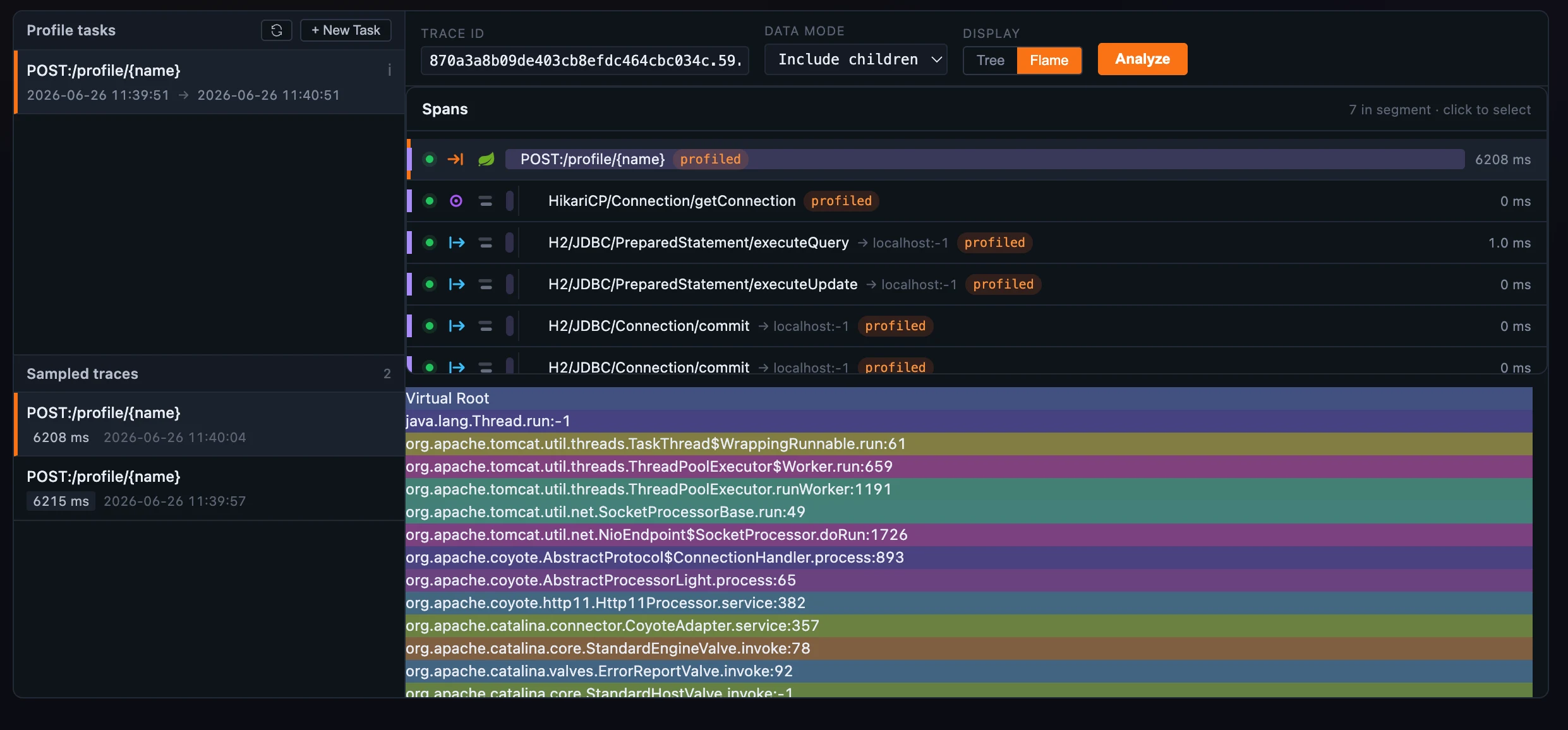 Figure 1: One flame graph for four profilers — frames by sample share, the selected frame pinned, the hover card with % of root.
On the Trace and eBPF tabs you can flip the same data to a Tree view instead — an indented stack table with each method’s total vs self duration and its dump count, expandable frame by frame. (Async and pprof are flame-graph-only; the toggle shows up where both views apply.)
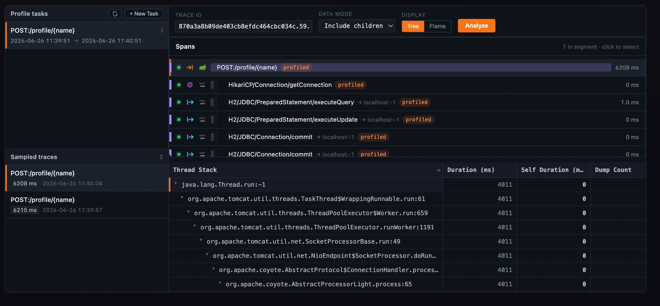 Figure 2: The same result, one toggle away — the Tree view swaps the flame for an indented stack table carrying total vs self duration and dump count.
What each of the four catches
The four stack profilers share the renderer but answer different questions, and each has its own New Task form:
- Trace Profiling samples the call stacks of slow trace segments. Scope a task to a service (and optionally one endpoint), set a slowness threshold and a dump period, and the agent snapshots thread stacks from segments that cross the threshold. Then you pick a sampled trace, drill to a profiled span, and Analyze — with a data mode that includes or excludes child-span time.
- Async Profiling runs the JVM async-profiler against a live Java service with no restart. A task can target several instances and several events at once —
CPU,ALLOC,LOCK,WALL, and the timer events — and an event-type selector re-draws the flame for whichever one you want to read. - eBPF Profiling captures kernel-level stacks with no in-process agent, driven by SkyWalking Rover: ON_CPU (where the process burns CPU) or OFF_CPU (where it’s blocked — on locks, I/O, scheduling). A process picker lets you expand a process’s attributes and pin the ones to profile, and an aggregate toggle counts samples or sums blocked time (the latter only makes sense off-CPU).
- pprof profiles a live Go service through the standard runtime profiler — exactly one event per task, chosen from
CPU,HEAP,BLOCK,MUTEX,GOROUTINE,ALLOCS, andTHREADCREATE. The dialog adapts to the choice: a duration for the timed captures, a sampling rate forBLOCK/MUTEX, and a one-shot snapshot for the rest.
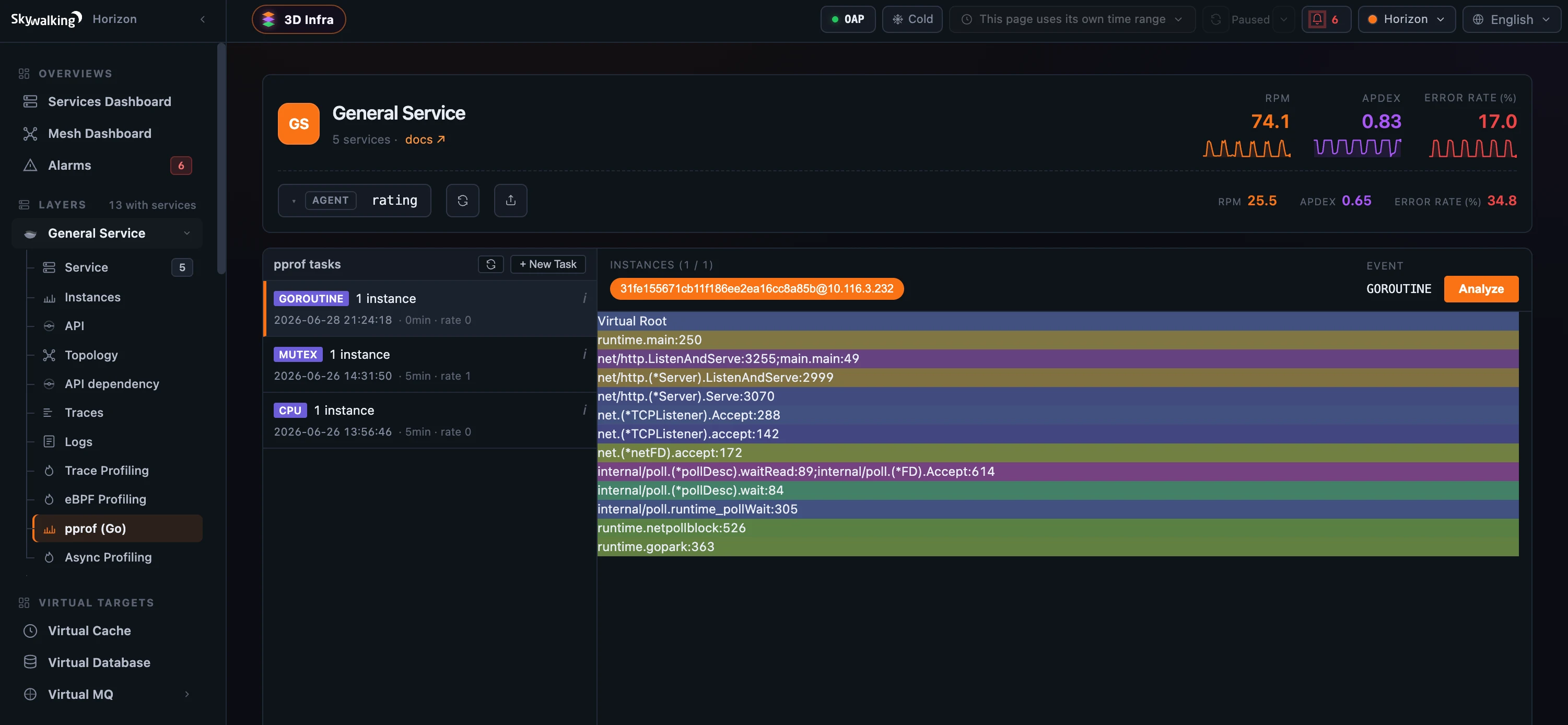 Figure 3: pprof takes exactly one Go event per task — GOROUTINE, MUTEX, and CPU are separate tasks, each with its own duration and sampling rate; select one and Analyze pours it into the same flame graph.
Network Profiling: the deliberate exception
The fifth profiler answers a different kind of question — not “where is one process spending time” but “which processes are talking to which, and over what” — so it renders differently on purpose. Network Profiling captures the network conversations between the processes of a service instance and draws them as a honeycomb topology: each process is a hexagon, the instance’s own processes pack into the centre under a dashed pod boundary, and external peers ring the edge. The links between them are directed and animated, and colored by protocol — HTTPS, TLS, HTTP, and plain TCP each get their own hue and a small pill.
It also runs differently: instead of a fixed duration, a network task carries sampling rules — match by URI pattern, by 4xx/5xx responses, or by a minimum duration, and choose how much of each request/response body to keep — and keeps running until you stop it. Click an edge and a Client side | Server side panel opens with that conversation’s call rate, latency, and bytes charted over the window. It’s drawn from the same process-relation data that powers the 3D Infrastructure Map — and there’s not a flame graph in sight.
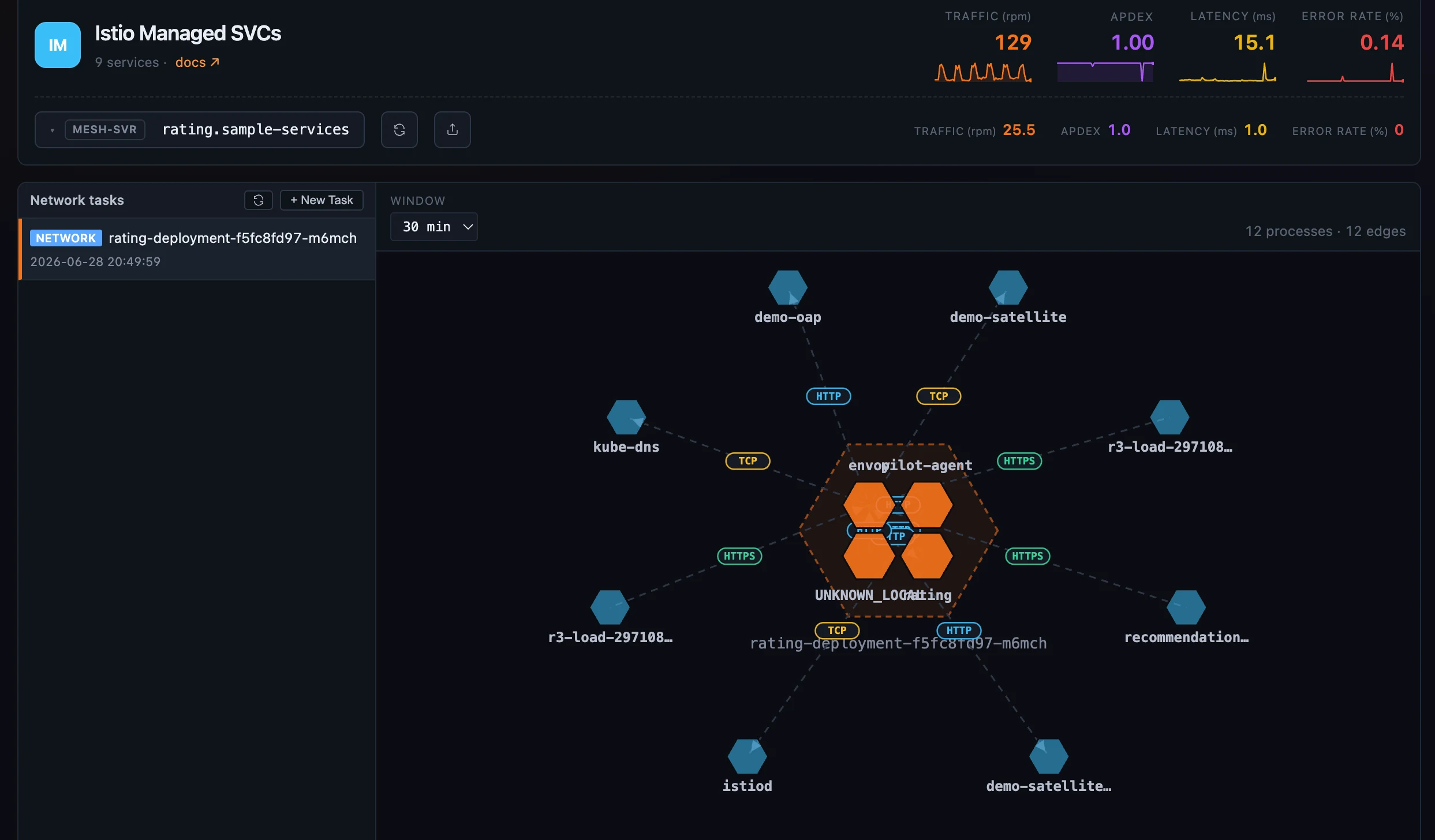 Figure 4: The odd one out — process conversations as a honeycomb. In-pod processes pack inside the dashed pod boundary, external peers ring it, and every edge is colored by protocol; clicking one opens its client-vs-server metrics.
One task model, two permissions
For all the differences in what they capture, every profiling tab is the same workflow: a task list on the left, a New Task control, and a result panel on the right. Create a task and the list polls for a few rounds until OAP has dispatched it and the instances report back; select a task to analyze it.
That create-versus-read split is also a permission boundary. Starting a task needs profile:enable (an operator-and-above default) — because an unbounded profile could peg a production instance’s CPU, so the task forms are duration- and size-capped on the server. Reading a result needs only profile:read (part of the read-only data catalog). So a viewer can sit with a flame graph all day and never be able to launch a profile.
Which tabs you even see depends on the service: a tab appears only when OAP reports that the service supports that kind of profiling. In practice the General agent layer carries the four stack engines (trace, eBPF, async, pprof), eBPF rides wherever Rover is deployed, and network profiling lights up on the service mesh.
Where to go next
For the field reference — every task field, the eBPF aggregate modes, the network sampling rules — see the Profiling docs.
Next up: Alarms & Incident Triage — the incident-centric alarm surface, and replaying the MQE snapshot that fired a rule.